Solving the Lasso Problem
Comparing optimization algorithms for Lasso
Introduction
Lasso regression is and important regularization technique for linear regression that can also perform variable selection. What this means is that solutions to the lasso problem tend to be sparse (contain zeros) which allows us to rule out certain independent variables in our model. A great resource to familiarize yourself with lasso is this video.
Lasso is of incredible importance in statistics, signal processing, compressed sensing, and image processing. In this post we will look at a variety of optimization technique for solving the lasso problem.
The lasso optimization problem is an unconstrained optimization problem which can be written as follows:
\[\begin{split} \underset{x}{\text{minimize}} \quad & \frac{1}{2}\|Ax-b\|_2^2 + \lambda \|x\|_1 \\ \end{split}\]where $A \in \mathbb{R}^{m \times n}$
A first thought to solve this problem might be gradient descent, however the objective function is non-smooth (due to the l1 penalty), so we cannot use gradient descent. A second thought is to use subgradient descent, which is a generalization of gradient descent to non-smooth functions. This would work, but subgradient descent has an extremely slow worst-case convergence rate of $\mathcal{O}(1 / \sqrt{t})$ (meaning you need four times the iterations to double the accuracy) so we will look at better algorithms.
Reformulating as Quadratic Program
One of the easiest things to do would be reformulating this problem as a Quadratic Program (QP) as follows:
\[\begin{split} \underset{x}{\text{minimize}} \quad & \frac{1}{2}\|Ax-b\|_2^2 + \lambda \sum_{i=1}^n t_i \\ \text{subject to} \quad & -t_i \leq x_i \leq t_i \quad \forall i \in [1,n] \end{split}\]To see how this was done reference the Mosek Modeling Cookbook
We can then feed this into a QP solver such as OSQP and then get an answer. This works, but it feels wasteful to turn an unconstrained problem into a constrained one and then use a generic QP solver. There should be better algorithms that exploit the structure of our problem where we have a smooth plus a non-smooth term.
ISTA
ISTA or iterative shrinking threshold algorithm is an application of the proximal gradient method to the Lasso problem.
The proximal gradient method solves problems of the following form, where $f$ is differentiable
\[\begin{split} \underset{x}{\text{minimize}} \quad & f(x) + g(x) \\ \end{split}\]The algorithm looks as follows:
\[x_{k+1} = \boldsymbol{\text{prox}}_{\eta g}(x_k - \eta \nabla f(x_k))\]where $\eta$ is the gradient descent stepsize for $f$ which will be the inverse of the Lipschitz constant of $f$.
The proximal operator $\boldsymbol{\text{prox}}_{\eta g}$ is a generalization of the projection operation and is defined as follows
\[\boldsymbol{\text{prox}}_{\eta f}(v) = \underset{x}{\text{argmin}} \left(f(x) + \frac{1}{2\eta}\|x-v\|_2^2\right)\]You can think of the proximal operator as returning a point which balances minimizing the function and staying close to the current point. The proximal operator for many function are well known in closed form. For more information on proximal operators and algorithms using proximal operators, refer to
The idea behind the proximal gradient method is to perform a gradient descent step assuming we are just going to be minimizing the smooth function $f$ and then do an evaluation of the proximal operator for $g$ which can be interpreted as a gradient descent step on the smoothed version of $g$. More technically we do a gradient descent step on the Moreau envelope of $g$.
Alternating between these two steps, we eventually minimize our original objective function.
For Lasso we will take,
\[\begin{split} f(x) &= \frac{1}{2}\|Ax-b\|_2^2 \\ g(x) &= \|x\|_1 \\ \end{split}\]It can be shown that the proximal operator for the l1 norm is the soft threshold operator
\[\boldsymbol{\text{prox}}_{\eta \|\cdot\|_1}(v) = \mathcal{S}_\eta(v) = \text{sign}(v)\max(|v|-\eta,0)\]We can now write out the ISTA iterates as follows
\[x_{k+1} = \mathcal{S}_{\lambda/L}\left(x_k - \frac{1}{L}A^\top(Ax_k-b)\right)\]Where $L$ is the maximum eigenvalue of $A^TA$. This can quickly be computed via power iteration.
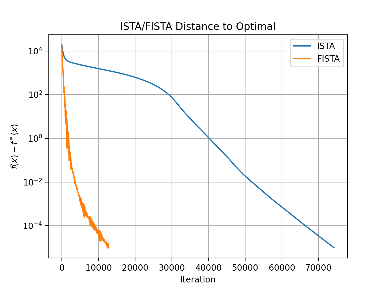
It can be shown that this algorithm has a worst-case convergence rate of $\mathcal{O}(1 / t)$ meaning that if we double the number of iterations, we double the accuracy of the solution. This is already better than subgradient method, but is not the best we can do.
FISTA
ISTA was used for a while, but many researchers noticed that it can be painfully slow to converge. In 2009, Beck and Teboulle introduced FISTA (Fast Iterative Shrinking Threshold Algorithm) where they used momentum to accelerate ISTA and were able to achieve the worst-case convergence rate of $\mathcal{O}(1 / t^2)$ , meaning that if we double the number of iterations, we quadruple the accuracy of the solution
This algorithm can be written as follows
\[\begin{align} x_k &= \mathcal{S}_{\lambda/L}\left(y_k - \frac{1}{L}A^\top(Ay_k-b)\right) \\ t_{k+1} &= \frac{1+\sqrt{1+4t_k^2}}{2} \\ y_{k+1} &= x_k + \left(\frac{t_k-1}{t_{k+1}}\right)(x_k-x_{k-1}) \end{align}\]ADMM
The final algorithm we will consider for Lasso is the Alternating Direction Method of Multiplers (ADMM). This algorithm was introduced in the mid-1970s, but became popular again after Stephen Boyd et al published their paper in 2011
The iterates of the algorithm are as follows:
\[\begin{align} x_{k+1} &= \underset{x}{\text{argmin}} \; \mathcal{L}_\rho(x,z_k,y_k) \\ z_{k+1} &= \underset{z}{\text{argmin}} \;\mathcal{L}_\rho(x_{k+1},z,y_k) \\ y_{k+1} &= y_k + \rho(x_{k+1}-z_{k+1}) \end{align}\]where
\[\mathcal{L}_\rho(x,z,y) = f(x) + g(z) + y^T(x-z) + \frac{\rho}{2}\|x-z\|_2^2\]For the case of Lasso, we have
\[\begin{align} f(x) &= \frac{1}{2}\|Ax-b\|_2^2 \\ g(z) &= \|z\|_1 \end{align}\]and the ADMM iterates become
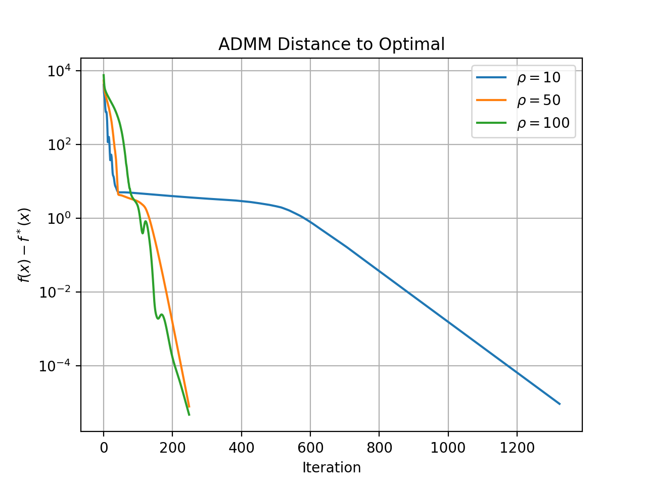
\[\begin{align} x_{k+1} &= (A^TA+\rho I)^{-1}(A^Tb+\rho z_k -y_k) \\ z_{k+1} &= \mathcal{S}_{\lambda/\rho} (x_{k+1}+y_k/\rho) \\ y_{k+1} &= y_k + \rho(x_{k+1}-z_{k+1}) \end{align}\]Here, $\rho > 0$ is a stepsize.
Results
Now we will test the QP version of Lasso, ISTA, FISTA, and ADMM to see which is fastest. To generate the data, I generated a random $A \in \mathbb{R}^{m \times n}$ with $m < n$, then generated a random sparse vector $x_{*}$, and calculated $b=Ax_*$.
The stopping criteria for all solver was coming within $0.0001$ of the optimal objective function value.


| Algorithm | Solve Time (sec) |
|---|---|
| ADMM (rho=50) | 0.197 |
| ADMM (rho=100) | 0.202 |
| ADMM (rho=10) | 1.097 |
| FISTA | 1.652 |
| OSQP | 2.271 |
| ISTA | 8.880 |
It should be mentioned that the ISTA, FISTA, and ADMM implementations are quite naive and unoptimized, but the OSQP solver is written is pure C. The slowest algorithm by far is ISTA followed by reformulating Lasso as a QP and using OSQP, followed by FISTA, and the fastest algorithm was ADMM. The code to generate the plots can be found here.